Metrology for Precision Motion / Positioning Systems - Methods and Principles
Part 2: How to Consistently Verify the Performance of Nanopositioning Motion Control Equipment
PI has been actively involved with a group of international engineers and scientists working on a new measurement standard that would better characterize the accuracy and performance of nano-positioning and high precision motion control systems, exceeding the ASME B.5.54 guidelines. While the work is still ongoing and different types of motion and positioning systems call for different test parameters to provide meaningful information regarding the applicability to the specific applications they were designed for, the information below describes the methodology employed by PI test engineers to ensure consistent product performance and quality. In Part 1 of this article, we discuss the necessary test and metrology equipment for high quality measurements.
1 Qualification of Positioning Equipment
Measurements are carried out on prototypes, individual products, and series-production products to qualify the positioning axes produced by PI (Physik Instrumente). In the case of series-production products, valid specifications are derived based on these measured values and then published in the datasheets. These specifications describe the fundamental positioning characteristics for a product type, such as e.g. positioning accuracy, angular error in multiple axes, and unidirectional and bidirectional repeatability.
It is important particularly in the design of customer-specific solutions that there is a common understanding of what the specifications are because it is only in this way that the design can be clearly defined.
This post describes:
- which measurements are carried out and which measurement methods are used
- which standards are considered to this process
- how the data acquired from the measurements is prepared
- how measurement results are derived from the data and what terminology is used to describe them
In addition, this post provides a brief overview of the measurement protocol and the measurement results that are reported and how both are structured.
2 Applicable Standards and Special Features of Precision Positioning
The measurement rules described here are mainly based on the ISO 230 series of international standards, whereby the standards ISO 230-1 (2012-03) and ISO 230-2 (2014-05) are primarily relevant, as well as the American standard ASME B5.54 (2005). This standard is to a large extent identical to the ISO 230 series of standards with respect to the measurements described in this document.
A major disadvantage of the stated standards for the qualification of micropositioning and nanopositioning systems is the fact that they were designed for larger turning lathes, milling machines, and similar products. Therefore, the explanations and detailed descriptions for the methods described in these standards are not always applicable for the qualification of products that are produced for high-precision micropositioning and nanopositioning. If it was not possible to transfer the ideas from these standards directly to the qualification of PI products, the measurement rules described in these standards were modified.
This means that the measurement rules used at PI are not a direct copy of the stated standards but rather they include specific adaptations and, in particular, enhancements of them with the aim of being able to test micropositioning and nanopositioning axes in the best way possible.
PI actively takes part in the current ASME B5.64 standardization committee which works on the development of a measuring standard for micro and nanopositioning systems.
3 Basic Measurement Procedure and the Measuring Equipment Used
3.1 General Measurement Procedure
Positioning axes (linear, rotary) are designed for a specific travel range.
Definitions: The travel range is the range within which the controller can move the system to different positions. The measuring range lies within this travel range or corresponds to the maximum travel range. The end points on each measuring range are always approached unidirectionally. All other measurement points can be approached bidirectionally. The classification "unidirectional" indicates a measurement series in which the movement to a target position is always carried out in the same direction, while "bidirectional" indicates that the movement to a target position is from both directions (forwards and backwards).
In order to determine a measurand, positions within the travel range are approached bidirectionally and a measurement is taken at the position. This is not possible at the end points of the travel range because these points represent the end of the numerically controllable range and these positions can only be reached coming from one direction. The so-called bidirectional measuring range excludes the end points and is thereby always a bit shorter than the entire measuring range. The data measured unidirectionally at the end points of the measuring range are only used for determining selected measurands. For example, this data is used to determine the stroke, which ensures that the positioning axes can also be traversed along the specified path.
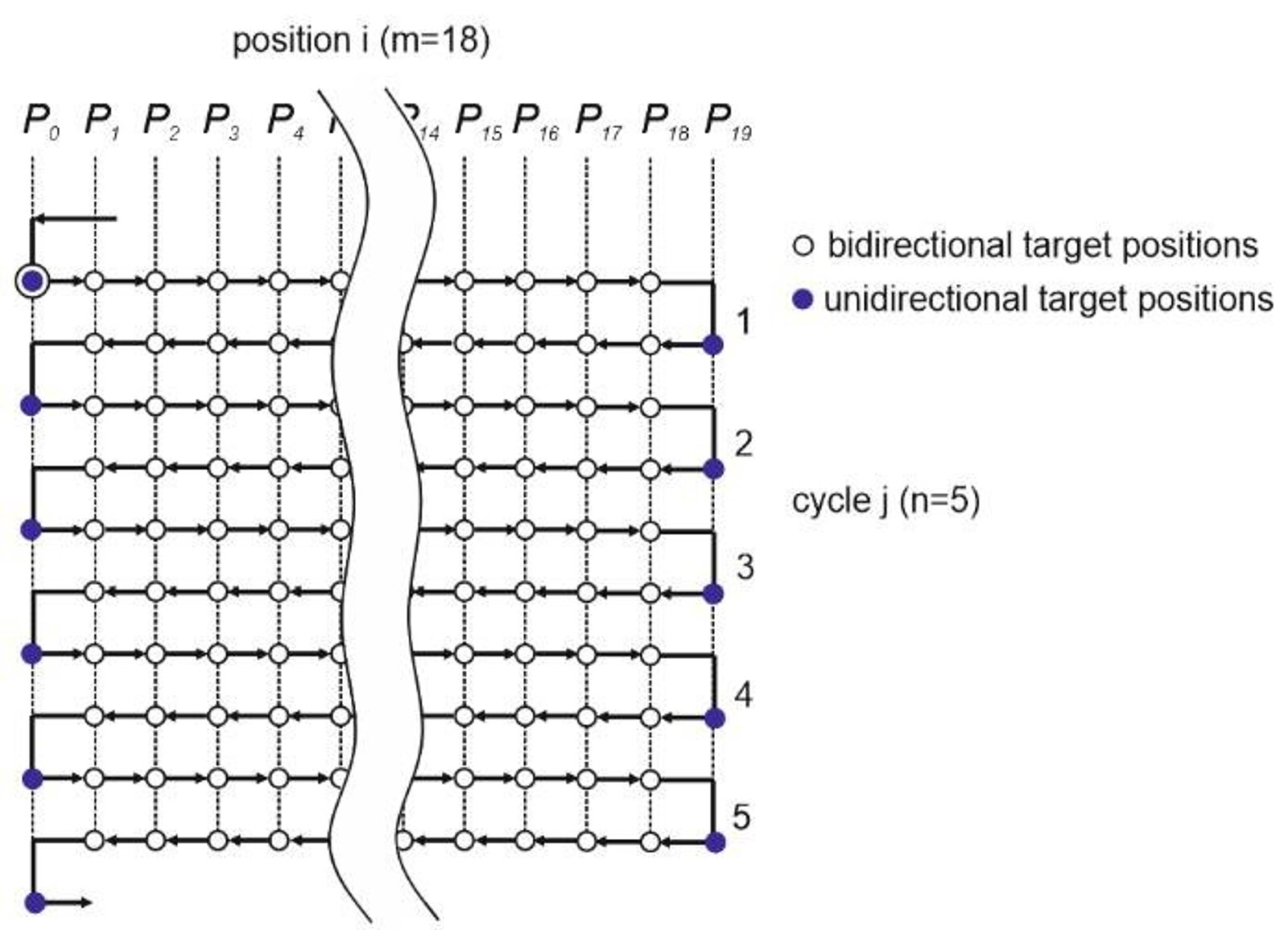
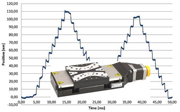
The positions within the measuring range at which measurement data are recorded are named target position Pi. As standard, target positions at the measurement points at the ends of the measuring range (two points) and another 18 points distributed equidistantly along the measuring range are measured, which makes 20 target positions in total. The axes are traversed to these target positions to record the measurement data in a meandering pattern (see Fig. 1) and the positioning data is recorded using suitable measuring equipment. The entire bidirectional cycle is completed five times as standard so that it is possible to record five sets of unidirectional measurements in both directions.
The entire measurement process only uses static measurements. This means that the axes are traversed to a target position, the moving platform is allowed to come to a standstill and only then is the measurement data recorded using corresponding measuring equipment.
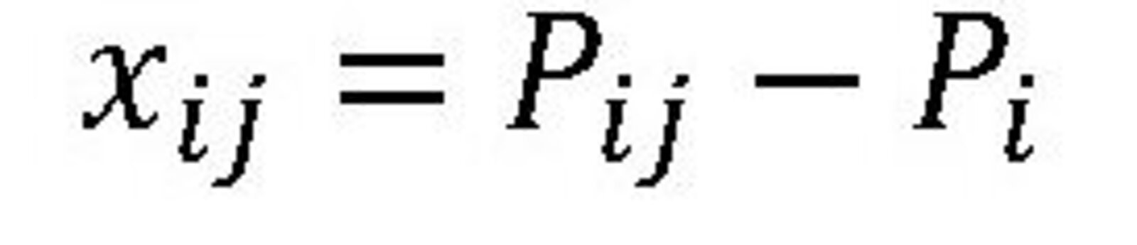
Using these measurements, the positioning error is calculated for every target position. These positioning errors xij↑ or xij↓ thus correspond to the difference between the current position actually reached Pij and the target position Pi. The corresponding positioning error is calculated for every cycle j at the target position i as follows:
3.2 Measuring Equipment
The measurement data is usually recorded using interferometers to determine the linear deflection and autocollimators to determine the angular error.
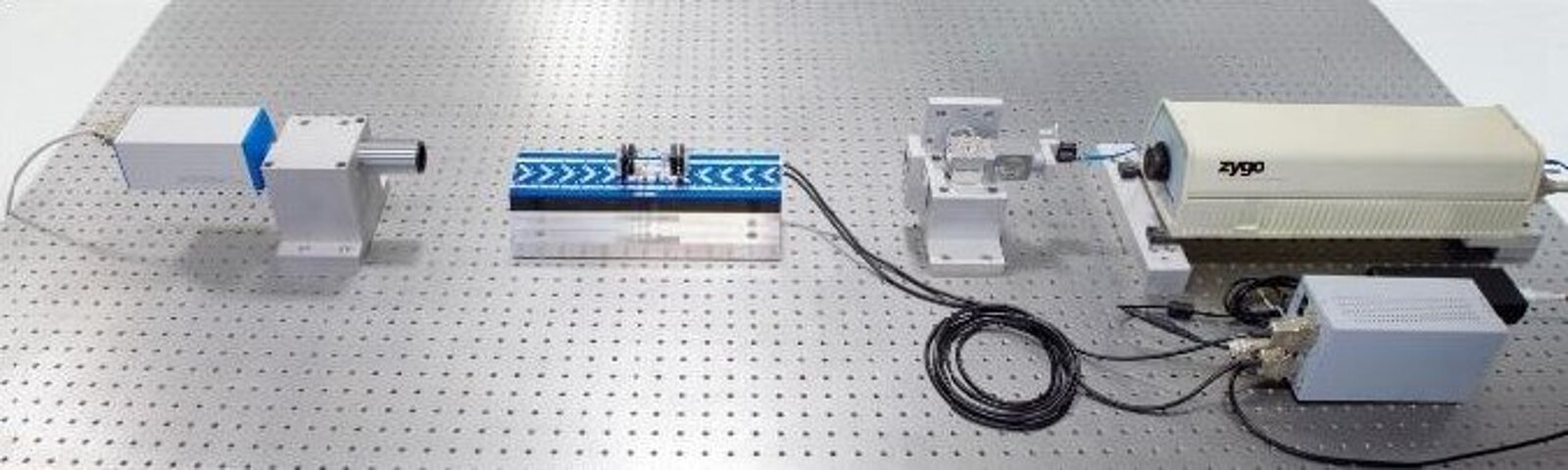
This type of setup is shown in Fig. 2. An interferometer is used from one direction to determine the linear displacement of the axis being tested, while an autocollimator is used to determine the angular error from the opposite direction at the same time. The positioning axis is equipped with two reflector mirrors, which are used by the interferometer and autocollimator for their measurements.
The measuring equipment used by PI is described in more detail in this blog: Metrology Equipment and Process for Qualifying Nanopositioning and Motion Control Systems
3.3 Correction of the Raw Data
3.3.1 Correction of the Abbe Error
An Abbe error occurs when an angular error has caused an error in the linear measurement (e.g. positioning accuracy).
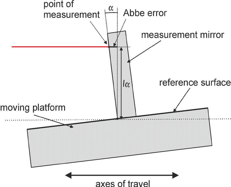
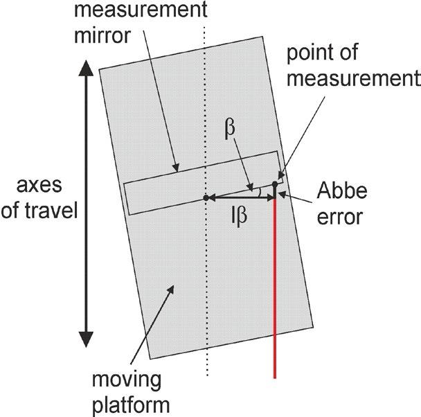
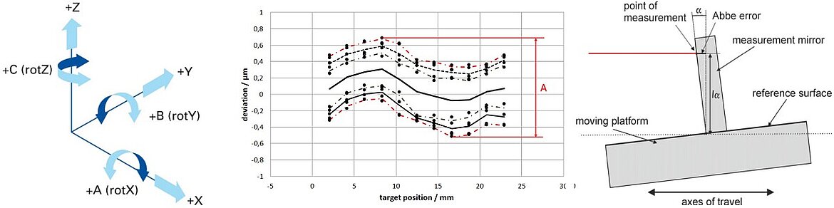
Fig. 3a, b: Abbe errors for both angles α, β: red = measuring beam, lα and lβ describe the distance to the axes with respect to the interferometer's measuring point. A correction is made to arrive at a point located at the surface of the moveable platform.
This is illustrated in Fig. 3: Due to the tilt of the moveable platform, there is an angular error when the beam from the interferometer hits the measurement mirror. The effect on the linear measurement value depends on the distance between the mirror and the platform. There is thus an error in the measurement value that can be corrected accordingly and eliminated from the data. Depending on the setup of the measuring equipment relative to the moveable platform, there can be an Abbe error in one or two directions. To calculate the correction, the linear measurement values are adjusted based on the angular data measured using the autocollimator. The distance between the moveable mirror and the surface of the moveable platform is determined and used for the calculation. This distance is also stated in the measurement protocol. Therefore, the measurement protocol shows whether or not a tilt correction of the measurement data has been carried out.
The angular and linear measurements are carried out separately from one another at PI. This means that the linear and angular errors can be distinguished from one another and are reported separately. If an Abbe error has been corrected during the test procedure, the surface of the moveable platform is used as the reference surface. The correction is calculated based on this. Using this information, the resulting positioning error for points at any distance to the platform can also be calculated.
3.3.2 Correction of Thermal Drift
It is not always possible to fully compensate for the influence of thermal fluctuations by monitoring and managing the ambient conditions. This is especially the case for positioning axes with resolutions and accuracies down to the subnanometer range. Even the smallest change in temperature during the measurement procedure can cause changes in position due to thermal expansion of the measurement setup or measuring equipment. Also, mechanical tension in the measurement setup and the resulting relaxation processes lead to such changes in position. If the highest level of accuracy is required, these effects can have a massive influence on the measurement results. Therefore, it may be necessary to correct for these thermal effects.
The measurement data is corrected based on the following assumptions:
- The positioning axis that is being tested does not itself change over time, except for the mechanical changes resulting from changes in temperature.
- If the temperature were stable, the first measurement point would always be measured at an identical position.
- Thermal drift is not position-dependent but rather time-dependent.
To make the correction, a straight line is calculated through the first measurement points of repeated sets of measurements taken one after another. This straight line (temporal) can then be subtracted from the measurement data for one set of measurements. This makes it possible to compensate for thermal drift.
The protocol indicates whether or not a correction has been carried out for thermal drift.
3.3.3 Linear Correction of Raw Data
If only the deviation from an ideal straight line is of interest for an evaluation, the raw data have to be initially corrected linearly. This means that a regression line is subtracted from the positioning error xij with respect to the commanded target position Pi. This is calculated according to the method of least squares.
The measurement protocol indicates whether or not a linear correction has been carried out.

4 Data Analysis
The calculation rules and the corresponding calculation formulae used to evaluate the measurement data are presented here.
4.1 Basic Data for the Positioning Error
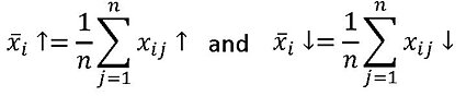
Firstly, the unidirectional positioning error is determined at every measured target position for both directions x̅i↑ and x̅i↓. This data is then used to calculate the mean positioning errors x̅i↑ and x̅i↓ for both directions at every individual position:
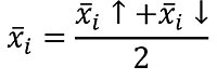
Using the mean positioning error at the points x̅i↑ and x̅i↓, which only measure the two individual directions (forwards and backwards), the mean value is determined. This is the mean bidirectional positioning error at every individual position xx̅ii:
The calculated values can be used to plot a mean curve that shows the mean errors of the axis across the entire travel range (see Fig. 4).
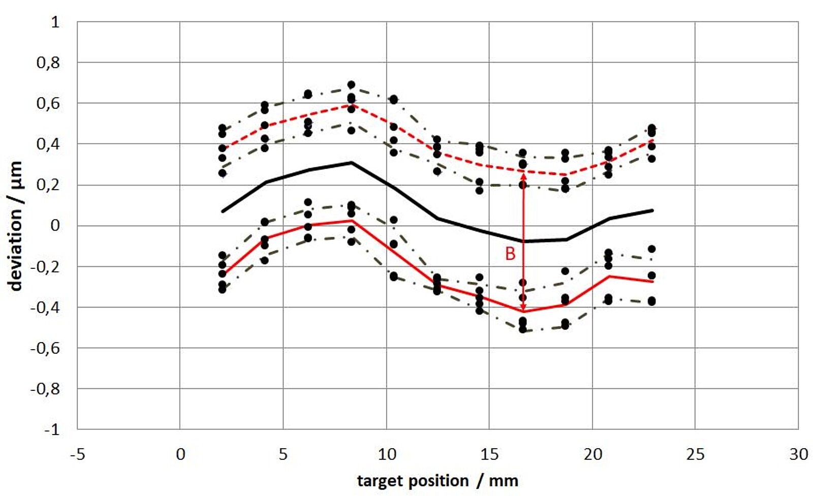
The mean values show the systematic deviation. Other variables for a positioning axis can be attributed to statistical deviations. For this reason, the standard deviations at the respective target positions Pi are determined separately for the forwards and backwards directions. This is carried out using the following formulae:
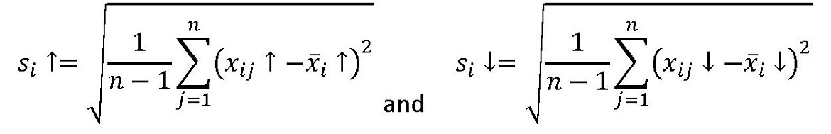
These five datasets together provide a good overview of the size of the statistical deviations and how the positioning axis behaves over the measuring range. Fig. 4 shows an example overview of the complete data. Other variables can be calculated on this basis.
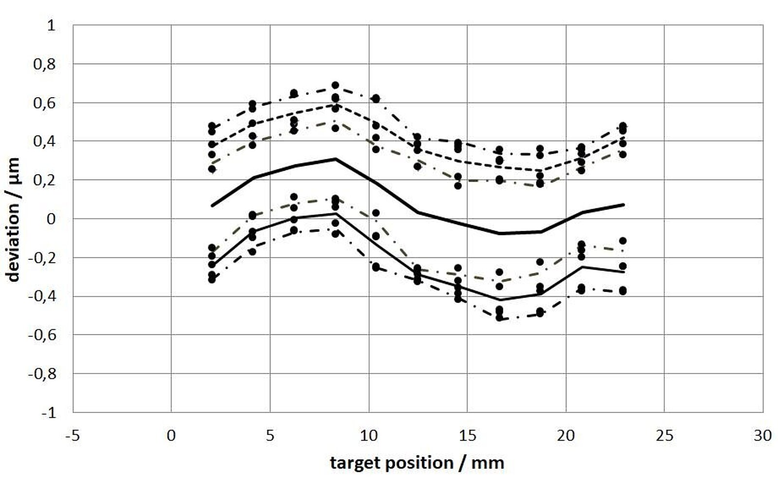
4.2 The Mean Bidirectional Positioning Error M
The mean bidirectional positioning error M is the difference between the maximum and minimum values for the mean bidirectional positioning errors at the points x̅i.
M = max(x̅i)−min(x̅i)
The mean bidirectional positioning error M is the maximum deviation (peak-peak) of the mean curve as described above, meaning the mean positioning error of the axis, see Fig. 5.
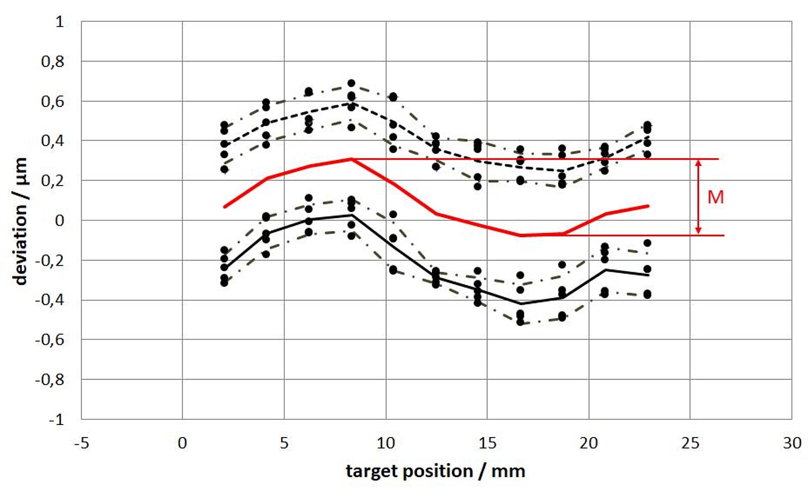
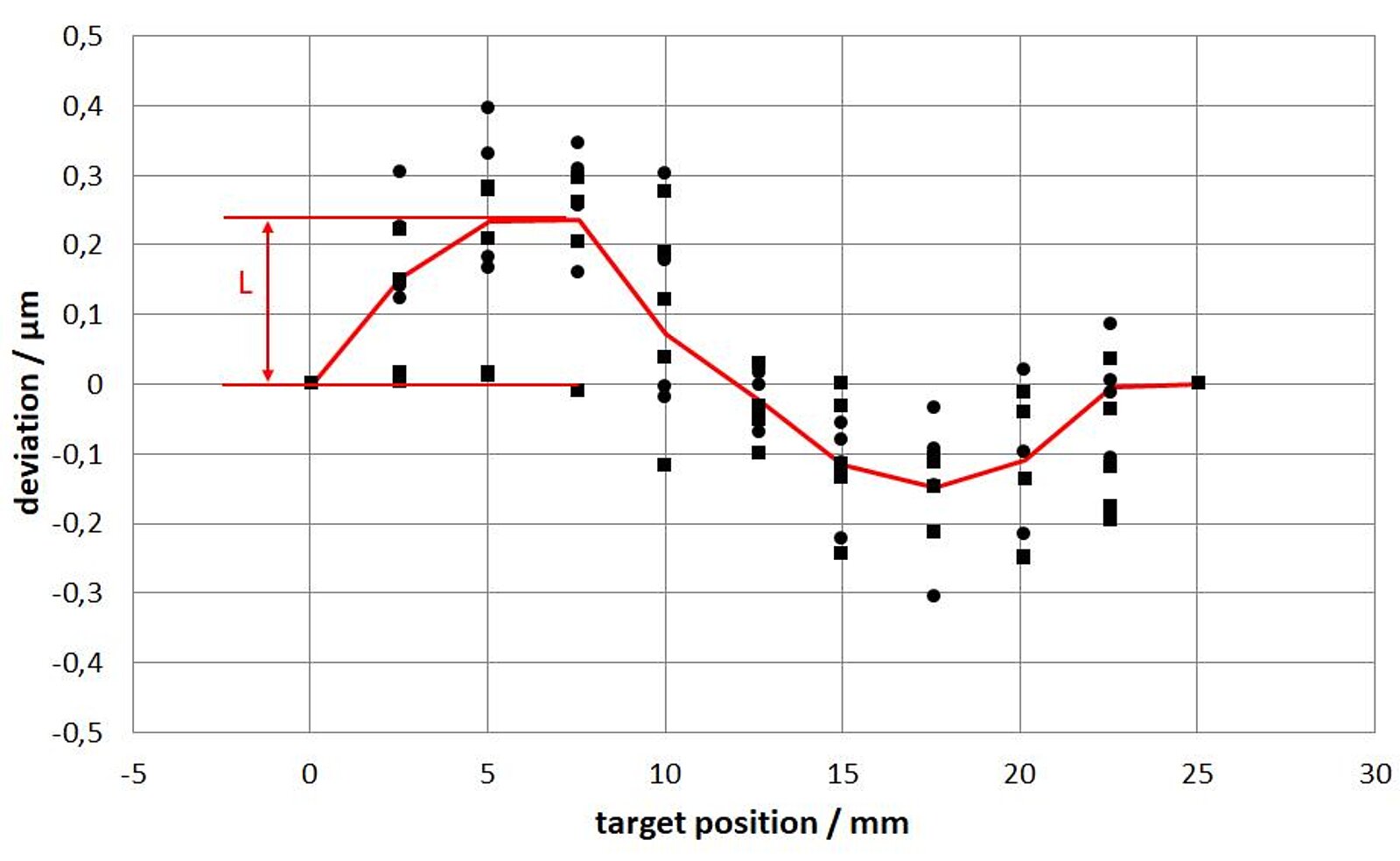
4.3 The Backlash B
To determine the size of the error between the positioning processes in the forwards and backwards directions, the maximum positioning backlash B is calculated. It represents the maximum deviation between the forwards and backwards directions.
B = max[|x̅i↑−x̅i↓|]
This is shown in red in Fig. 6.
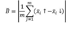
A mean backlash can also be determined on this basis. This indicates the size of the mean deviation between the forwards and backwards directions. To determine the mean positioning backlash B̄, the sum of the mean values for the backlash at all individual positions is determined as follows:
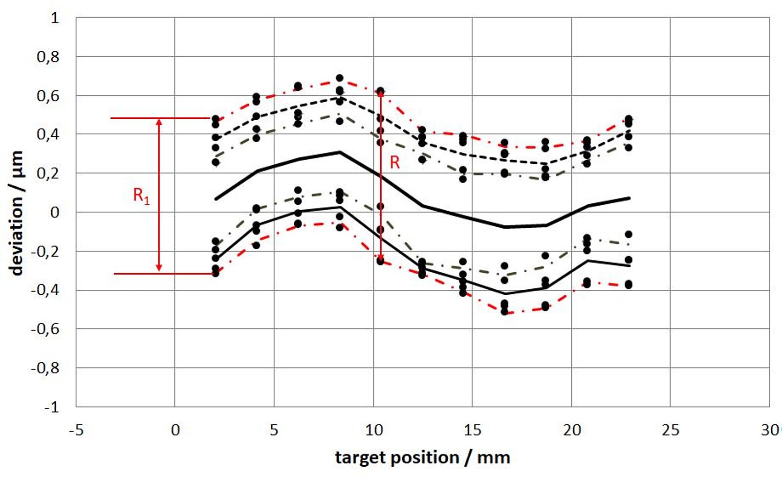
4.4 Unidirectional and Bidirectional Repeatability R
Another important characteristic of a positioning device is repeatability.
To calculate the repeatability, the bidirectional positioning repeatability Ri is first calculated for one position. It is calculated as follows:

The bidirectional repeatability indicates how "well" each individual target position will always be "hit" from different directions.
Accordingly, the maximum bidirectional repeatability is the maximum value of the repeatability values at the target positions:
R = max[Ri],
which is shown in Fig. 7
The maximum unidirectional positioning repeatability RR↓↑ is the maximum value of the standard deviations of the unidirectional repeatability for a positioning axis:
R↓↑ = ± max [si↑; si↓]
The maximum unidirectional repeatability indicates how large the maximum deviation at any target position can be when approaching the position from the same direction.
The value for the unidirectional positioning repeatability is given as a ± value.
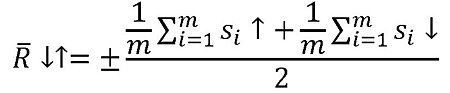
The average unidirectional positioning repeatability R̄↓↑ is calculated as follows:
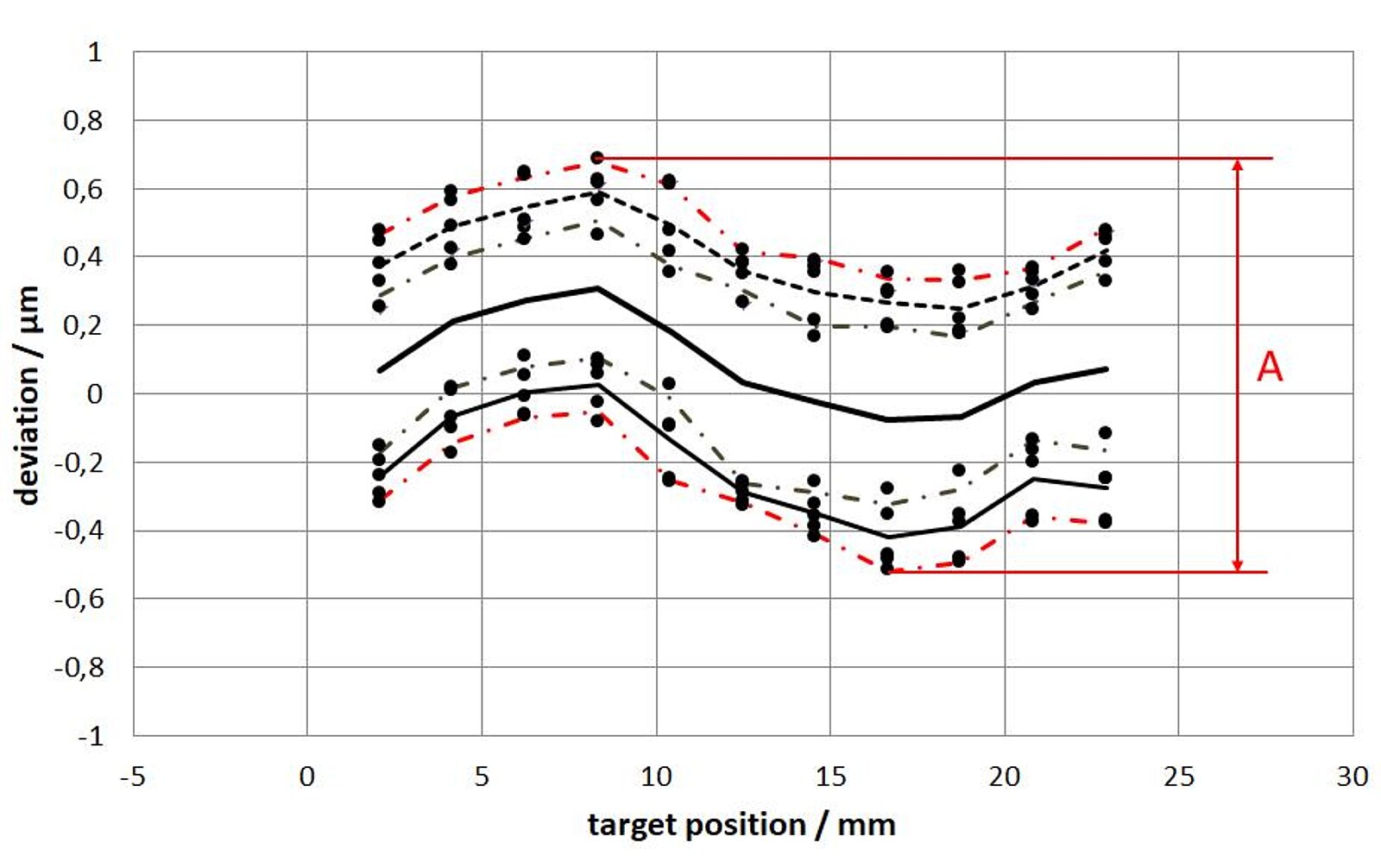
4.5 The Bidirectional Positioning Accuracy A
The bidirectional positioning accuracy A is a measurand that combines all errors that arise and thus represents the maximum error that can occur during positioning.
The bidirectional positioning accuracy is the range that is calculated by combining the bidirectional systematic deviations with the statistical deviations:

4.6 The Hysteresis H
The hysteresis H of an axis is the maximum difference of forwards and backwards values at all target positions:
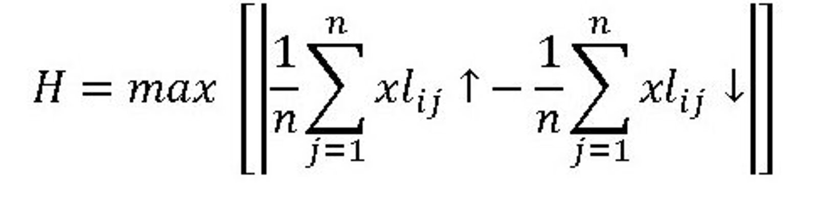
The calculation of H is carried out in the same way as the calculation of the backlash B. Accordingly, the percentage hysteresis Hp (in percent) is calculated as follows:
HP = 100 (H/LM)
5 The Coordinate Systems Used and Designations of the Axes of Motion
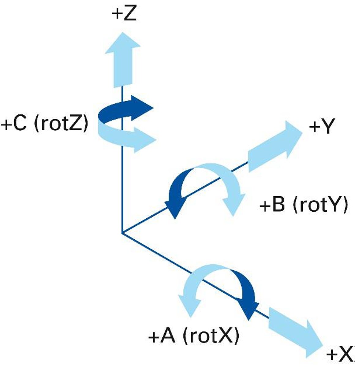
In general, PI uses a right-handed coordinate system to designate the axes of motion. The linear axes are thus labeled with X, Y, and Z and the rotational axes with A, B, and C. The rotational axes are assigned according to the linear axes, e.g. A is the rotational axis around the linear axis X.
In places where further clarification is necessary, the rotational axes are also labeled with an explicit reference to the linear axes, e.g. A (rot X). To illustrate how the axes are designated, the coordinate system is once again shown in Fig. 10.
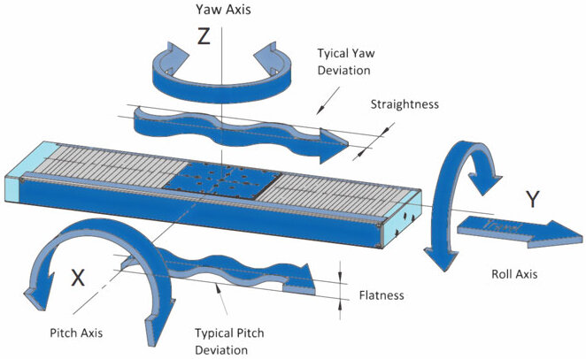
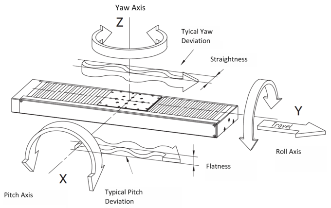
6 Mechanical Crosstalk of a Movement and Designation of the Error
In the case of mechanical positioning axes, it is usually not just the positioning error in the direction of motion that is relevant but also the mechanical crosstalk of a linear motion in the other linear and rotational directions. To determine this mechanical crosstalk, linear measurements orthogonal to the direction of motion and corresponding angle measurements are carried out. Here, a measurement is carried out according to the motion profile of the measurement procedure described in Section 3.1. The same methods as for the positional data are used to analyze these data. However, the analysis does not subtract the actual position from the target position but uses the raw data.
Straightness and flatness are calculated from the mean bidirectional positioning error after a linear correction ML has been carried out. It is still important to note here that the rotational error can transfer to a translational error at the functional point in certain circumstances, depending on where the zero point for the parasitic tilt lies. The errors themselves have a clear nomenclature. The various measurable errors for linear motion are shown in Fig. 11.
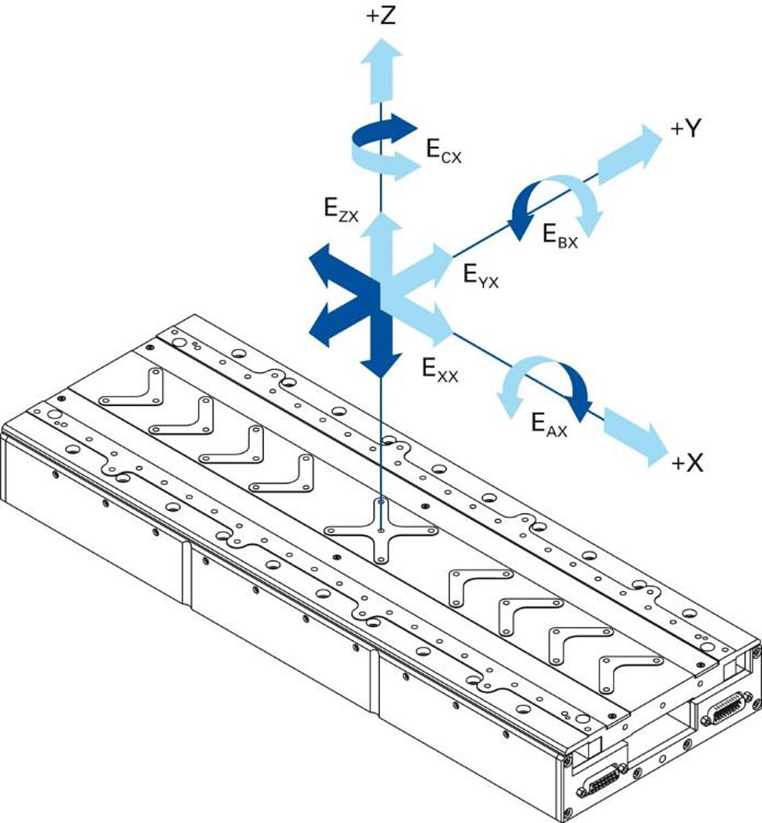
Fig. 11 Nomenclature of errors in the various axes for a linear motion:
E Axis designation where the error has been measured (commanded axis)
X Axis of the commanded linear motion
EAX Angular error around the X-axis (roll)
EBX Angular error around the Y-axis (pitch)
ECX Angular error around the Z-axis (yaw)
EXX Positioning error of the X-axis
EXXL Positioning error of the X-axis, minus regression line
EYX Straightness error in the direction of the Y-axis (straightness)
EZX Straightness error in the direction of the Z-axis (flatness)
If two axes are moving (e.g. X and Y), it is still possible for a combined parasitic motion to occur in the Z-axis. This error is called the out-of-plane error.
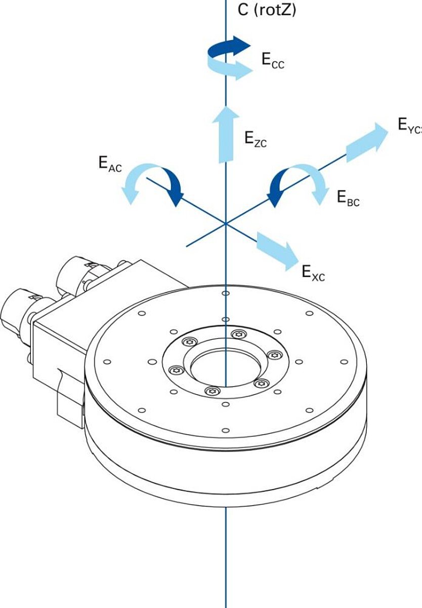
Fig. 12 Nomenclature of errors in the various axes for a rotary motion:
EXC Radial error in the direction of the X-axis
EYC Radial error in the direction of the Y-axis
EZC Axial error from C
EAC Tilt error around the X-axis
EBC Tilt error around the Y-axis
ECC Angular positioning error of C
A combined rotatory error, i.e. a radial error motion, is described as follows:
EXYC Radial error of C
Accordingly, a combined tilt deviation is referred to as follows:
EABC Tilt error of C
7 Additional Documents and Links


Blog Categories
- Aero-Space
- Air Bearing Stages, Components, Systems
- Astronomy
- Automation, Nano-Automation
- Beamline Instrumentation
- Bio-Medical
- Hexapods
- Imaging & Microscopy
- Laser Machining, Processing
- Linear Actuators
- Linear Motor, Positioning System
- Metrology
- Microscopy
- Motorized Precision Positioners
- Multi-Axis Motion
- Nanopositioning
- Photonics
- Piezo Actuators, Motors
- Piezo Mechanics
- Piezo Transducers / Sensors
- Precision Machining
- Semicon
- Software Tools
- UHV Positioning Stage
- Voice Coil Linear Actuator
- X-Ray Spectroscopy