1. Introduction
When building high precision positioning systems using our PIglide air bearing products, performing the metrology and testing is one of the most critical steps in the process. Only with proper metrology can we verify that our products and systems meet the specifications that our customers demand.
In this article, we discuss the various metrology tests performed at PI USA before we deliver a system to a customer.
2. Definitions: What Do We Test?
When working with linear motion, we typically have a fixed set of errors we want to define and measure.
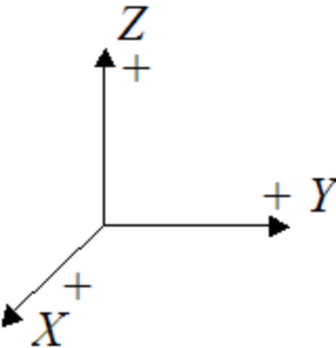
First, let’s define our coordinate system; X = axis of motion for a linear stage
Position accuracy is defined as the difference between the target position to which the system was commanded to move (in the X direction) and the actual position as measured by a metrology device.
Position repeatability is defined as the range of positions attained when the system is repeatedly commanded to one location under identical conditions. Repeatability can be defined in different statistical ways. In our case, we simply report the worst-case spread of points overall.
For the purposes of this article, we are defining position accuracy and repeatability in only the direction of travel, and not in 3D space. The other error motions described below account for the off-axis errors.
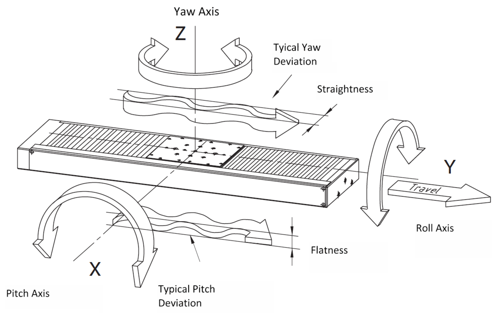
Pitch is defined as the angular error motion of the stage’s moving platform (or table) rotating about the Y axis.
Yaw is defined as the angular error motion of the stage’s moving platform (or table) rotating about the Z axis.
Roll is defined as the angular error motion of the stage’s moving platform (or table) rotating about the X axis. Roll is typically not tested.
Straightness error motion (“straightness”) is defined as error motion in the Y direction. As the stage travels along the X axis, the motion deviates from the perfect line by some amount.
Flatness error motion (“flatness”) is defined as error motion in the Z direction. As the stage travels along the X axis, the motion deviates from the perfect line by some amount.
When working with rotary motion, we use a different set of characteristics.
Positioning accuracy and repeatability follow the same definition as in the linear positioning section. The only difference is that the axis of motion is now angular instead of linear.
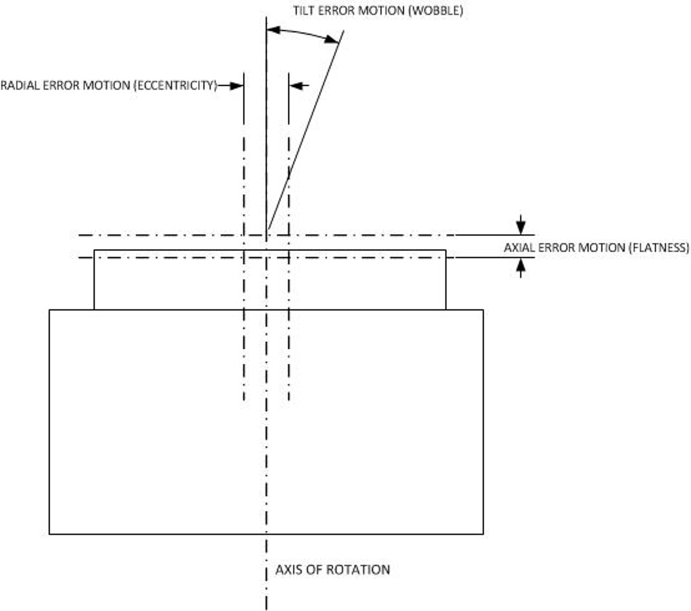
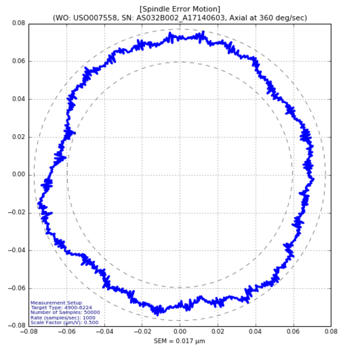
Axial error motion is defined as the linear error motion of a rotary stage in the direction of the axis of rotation. This error motion is sometimes also referred to as rotary flatness.
Radial error motion is defined as the linear error motion of a rotary stage perpendicular to the axis of rotation. This error motion is sometimes also referred to as eccentricity.
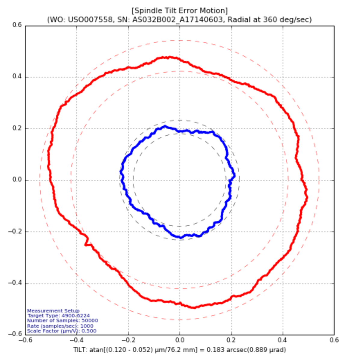
Tilt error motion as defined as the angular error motion of a rotary stage’s axis of rotation. This error motion is sometimes also referred to as wobble.
Rotary error motions are sometimes broken down into synchronous and asynchronous errors. Synchronous error motion is defined as the component of the total error motion that occurs at integer multiples of the rotation frequency. Asynchronous error motion is defined as the component of the total error motion that occurs at non-integer multiples of the rotation frequency. The two errors combined comprise the total error motion of the stage, which is typically the value we measure and report.
There can be additional specifications that must be measured in a particular system. These can involve dynamic performance like speed, acceleration, step and settle, and velocity regulation or other aspects like stability, minimum step size, resolution, and many more. For the purposes of this article, we limit the discussion to the error motions defined above.
3. Tools: How Do We Test?
We use two primary sets of tools at PI to measure all the error motions defined in the previous section: laser interferometers and capacitance probe sensors. Each test we perform varies slightly in the setup and the data collection method.
A detailed description of how these measurement tools work is beyond the scope of this article. For reference, see the following:
More information on interferometry
More information on capacitive sensing
3.1. Linear Positioning Accuracy and Repeatability
This test is performed with a retroreflector mounted to the stage’s moving table. The interferometer optic is placed at the end of the stage and is stationary. The mean path is in the direction of motion.
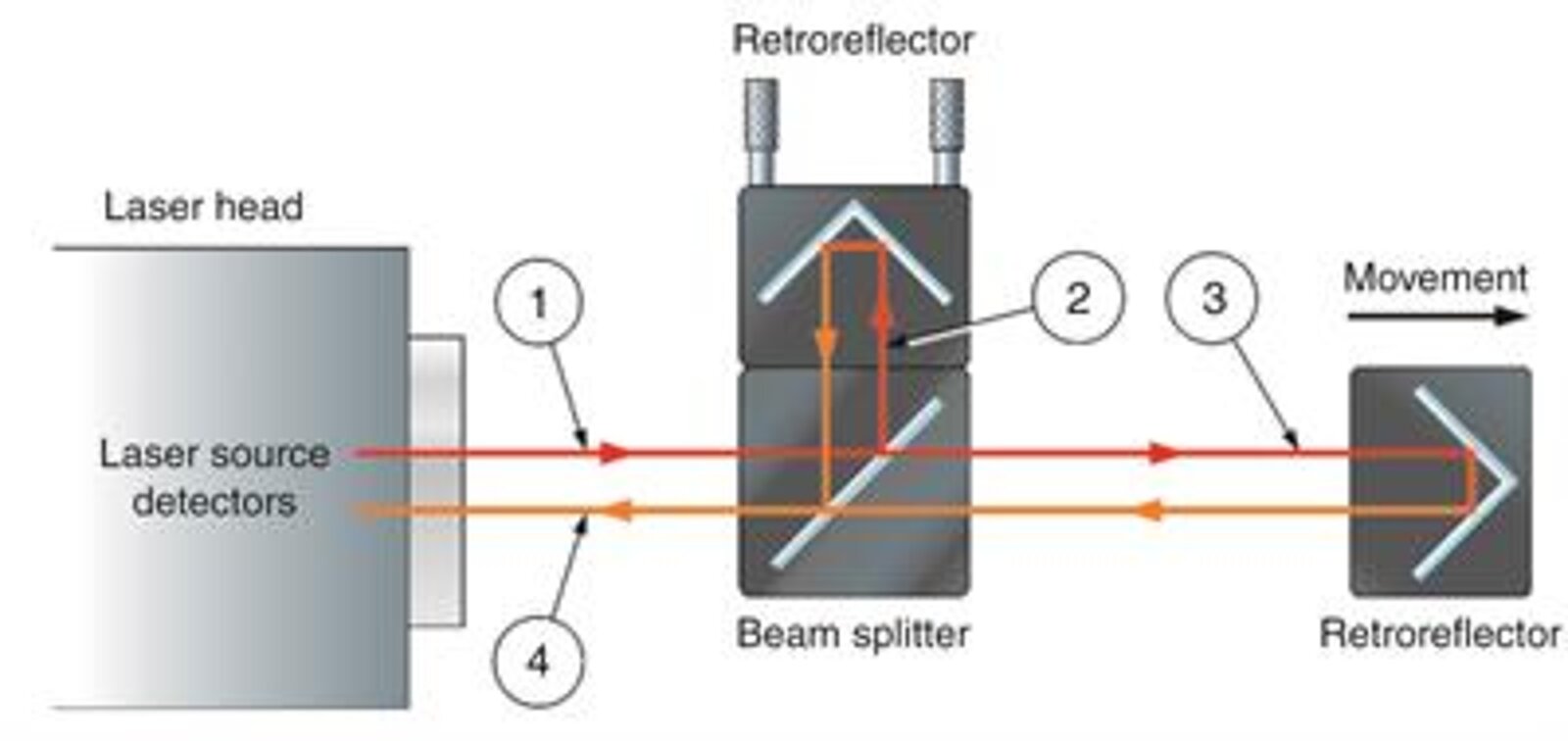
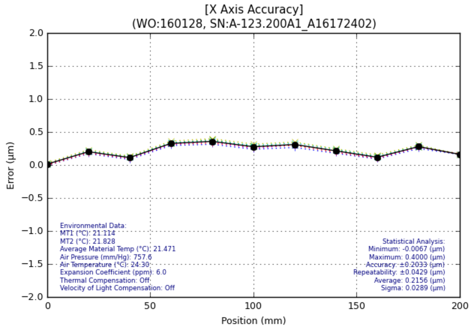
Under closed loop servo control, the stage is moved in fixed increments (typically 10mm – 50mm per step) and a measurement is taken at each point. The stage is moved through its full length of travel, in both directions, for multiple passes. The data that is collected is plotted and the overall accuracy and repeatability are calculated. The accuracy and repeatability results are typically reported in microns.
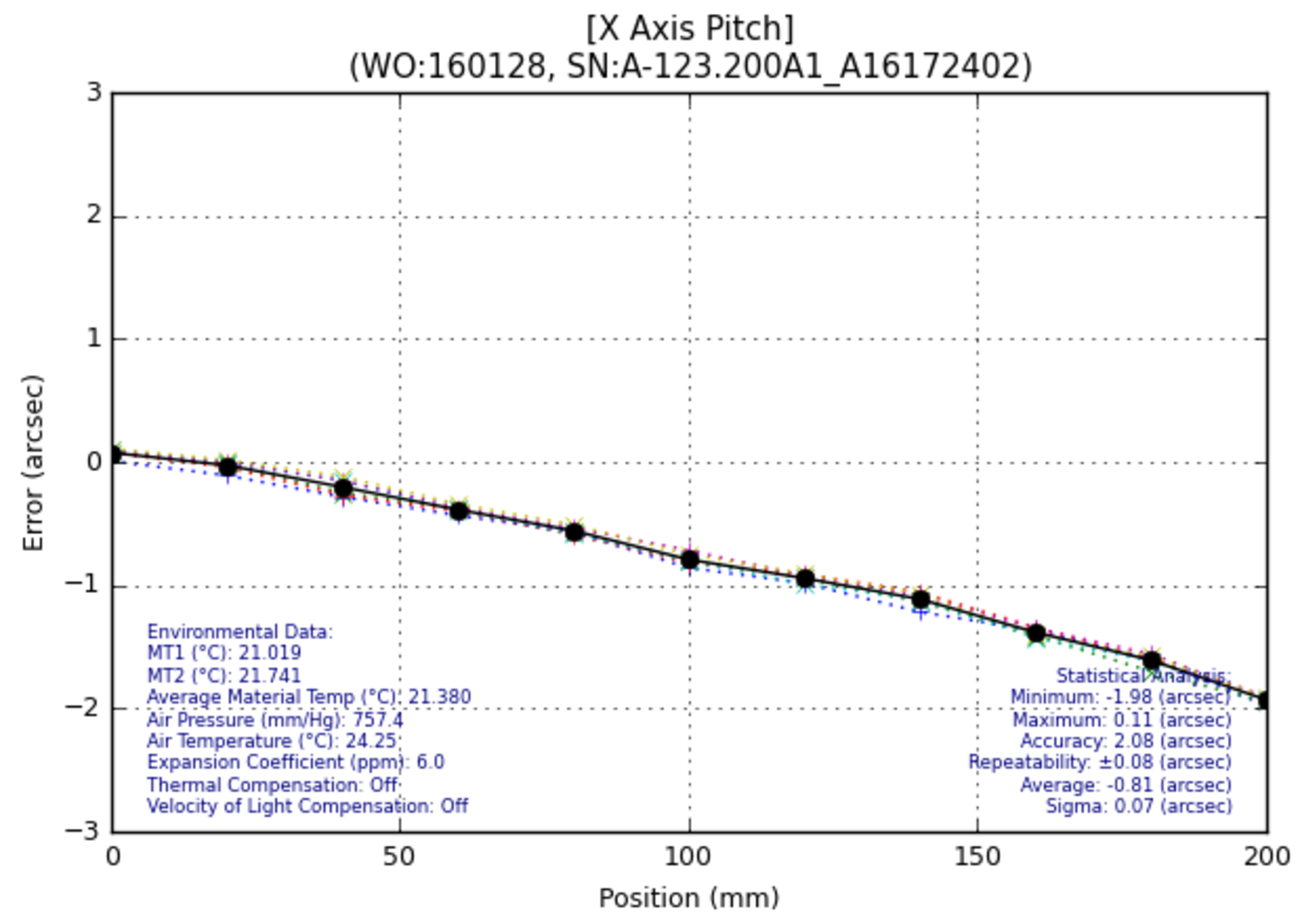
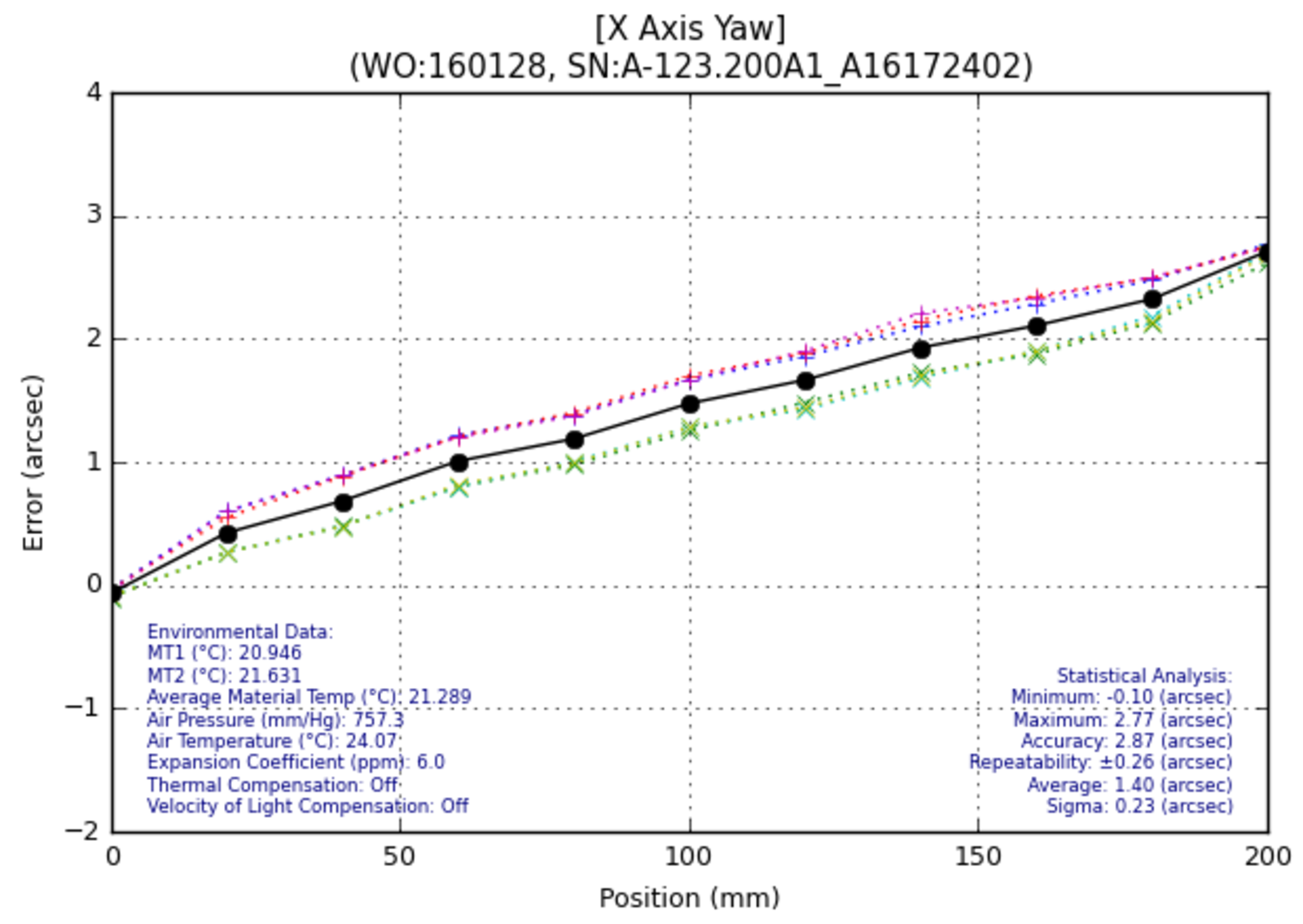
3.2. Pitch and Yaw
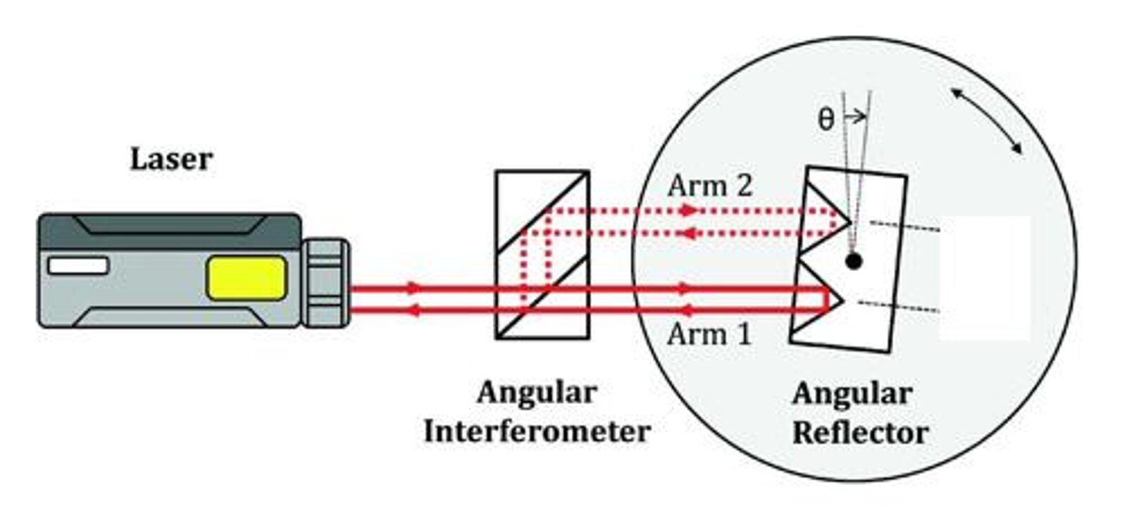
This test is performed with an angular retroreflector mounted to the stage’s moving table. The angular interferometer optic is placed at the end of the stage and is stationary. The mean path is in the direction of motion. The angular optic setup creates two beam paths. As the stage pitches or yaws, one beam arm will be longer than the other. The angular error is calculated based on the difference between the two signals. The only difference between the two test setups is the orientation of the optics.
In the same way as the accuracy data is collected, the stage is moved in fixed increments (typically 10mm – 50mm per step) and a measurement is taken at each point. The stage is moved through its full length of travel, in both directions, for multiple passes. The data that is collected is plotted and the overall errors are calculated. The results are typically reported in arc-seconds or microradians.

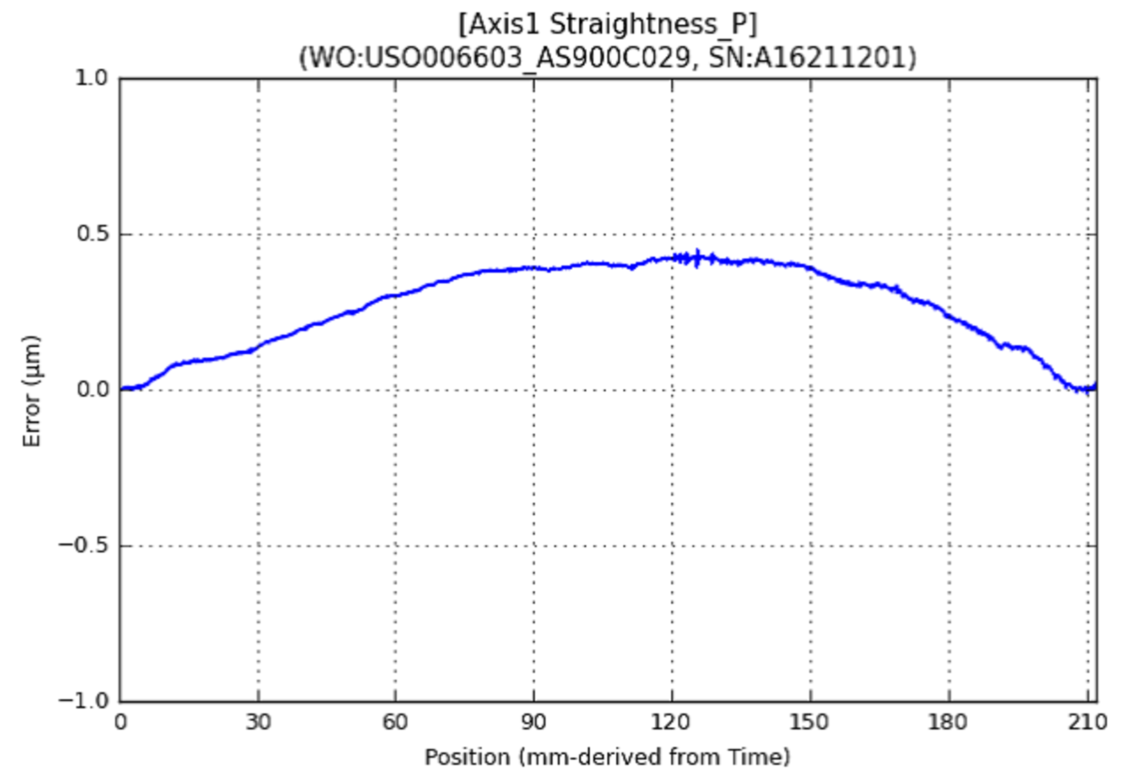
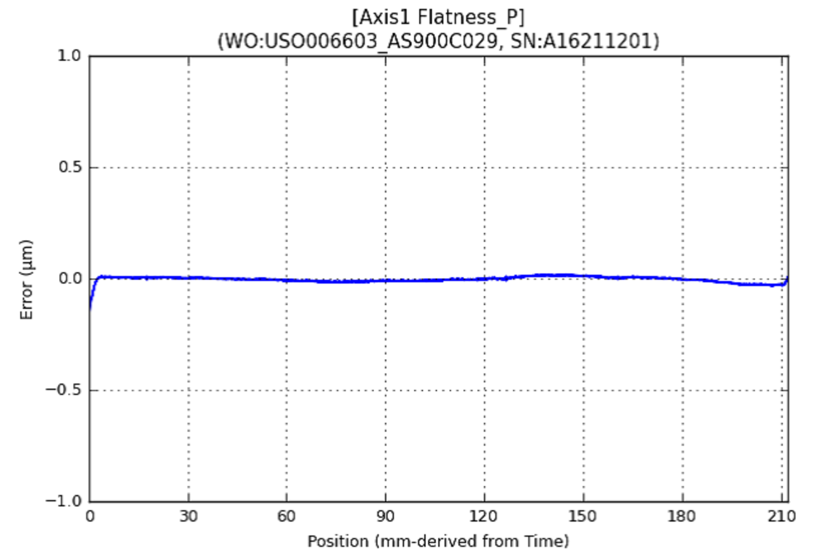
3.3. Straightness and Flatness
The straightness test is performed with a long plane mirror mounted to the stage’s moving table. The linear interferometer optic is placed next to the stage and is stationary. The mean path is orthogonal to the direction of motion.
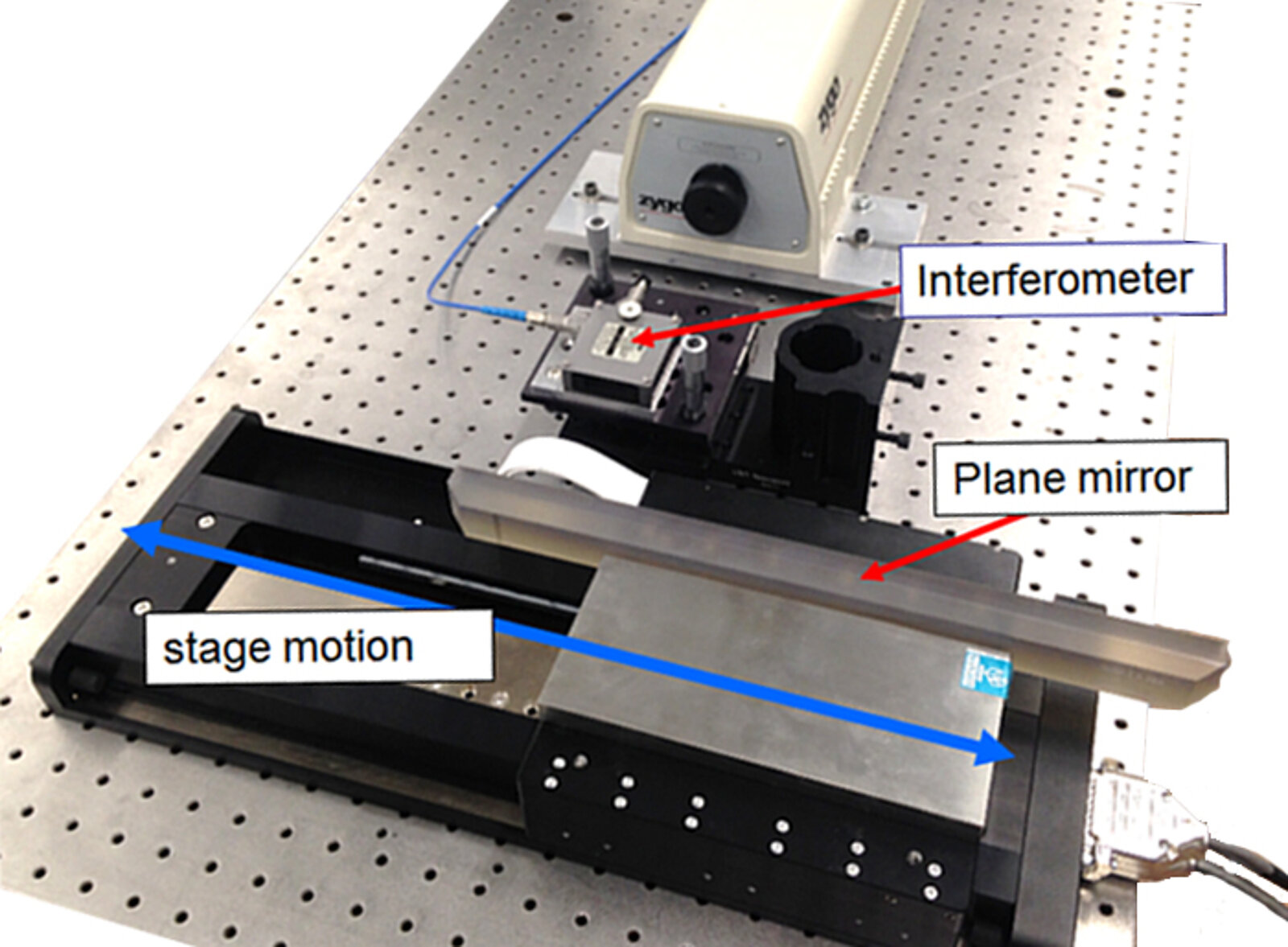
The flatness test setup is the same, except the orientation of the plane mirror and the beam path are rotated 90° so that the face of the mirror is horizontal and facing up.
Under closed loop servo control, the stage is moved at a constant velocity while data is collected from the laser at a fixed rate (usually 100 Hz – 20 kHz). The stage is moved through its full length of travel, in both directions, for multiple passes. The data that is collected is plotted and the overall error calculated. The results are reported in microns.
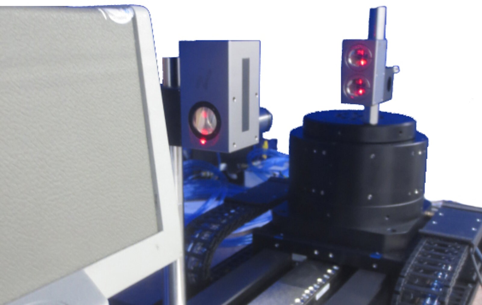
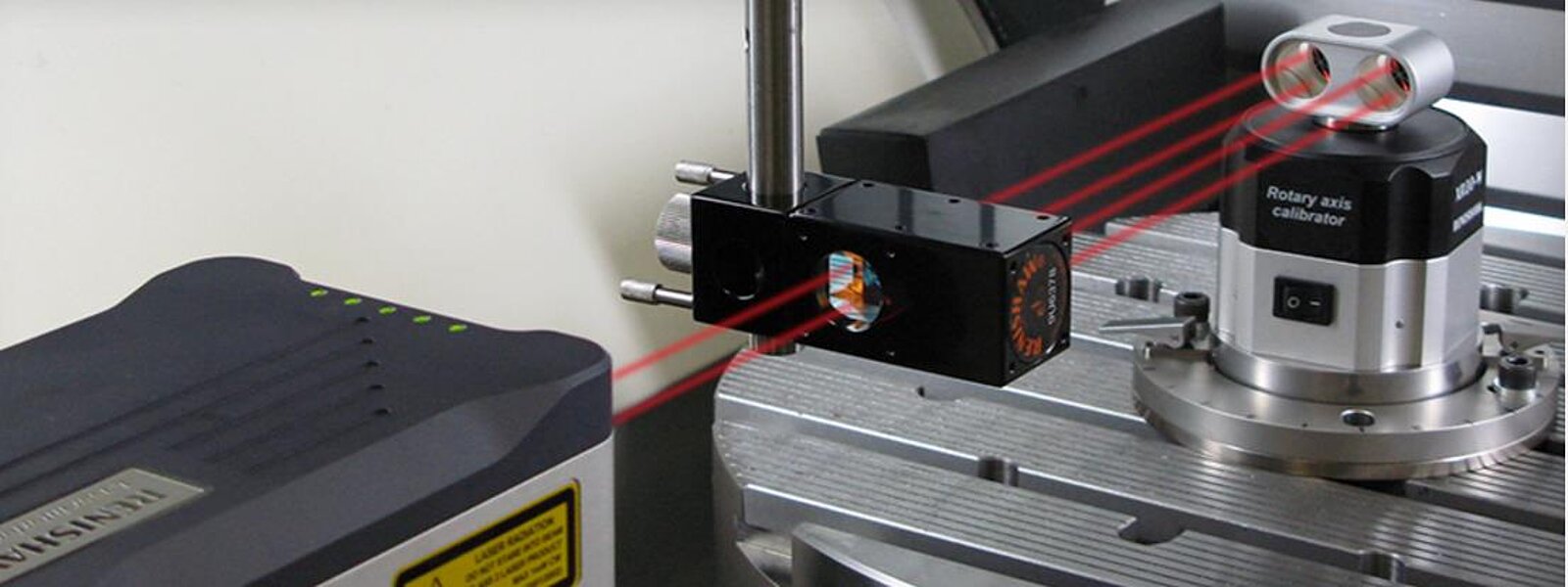
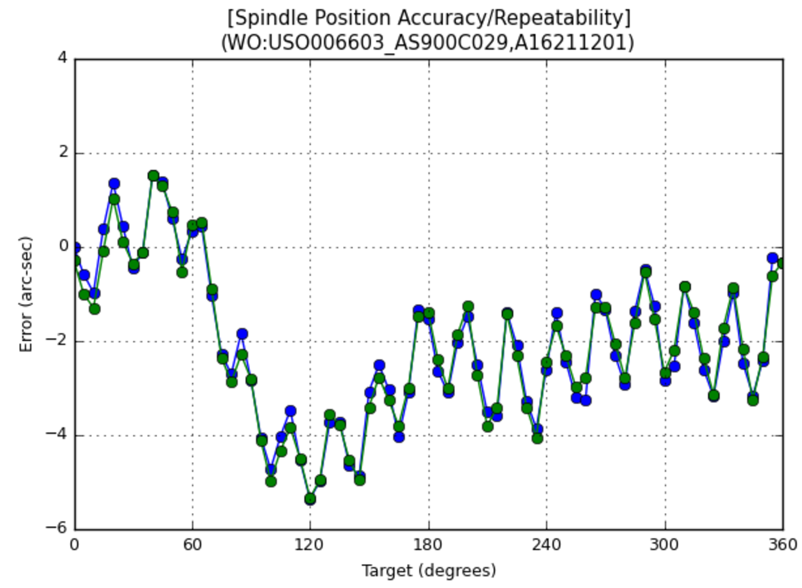
3.4. Rotary Positioning Accuracy and Repeatability
This test is performed using a similar optics setup as the yaw measurement test described earlier. However, additional hardware is required, since the yaw optics can only measure up to about 10° of rotation before the beam path is broken. To overcome this, we use a special rotary calibration mechanism mounted to the stage table.
To learn more about this tool, see http://www.renishaw.com/en/xr20-w-rotary-axis-calibrator–15763
In the same way as the linear accuracy data is collected, the stage is moved in fixed increments (typically 5° – 30° per step) and a measurement is taken at each point. The stage is moved through its full range of travel, in both directions, for multiple passes. The data that is collected is plotted and the overall errors are calculated. The results are typically reported in arc-seconds or microradians.
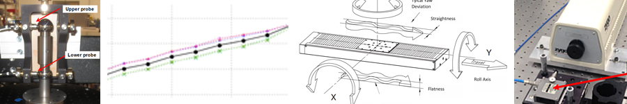
3.5. Rotary Error Motions
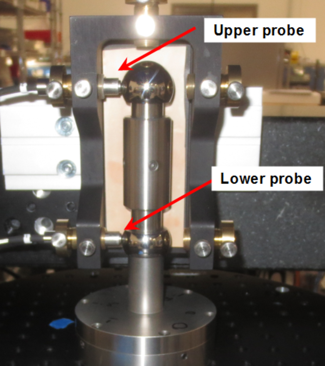
Unlike all the previous tests in which a laser interferometer is used, the tests for radial, axial, and tilt error motion in a rotary motion axis require the use of different tools. Here we use a mechanical artifact called a master ball. The steel ball is made to be almost perfectly round and spherical. The ball is mounted to the rotating table of the rotary stage, and stationary capacitive probes are used to measure the motion axially or radially of the ball as it spins. The only difference between axial and radial measurements is the orientation of the probe relative to the ball.
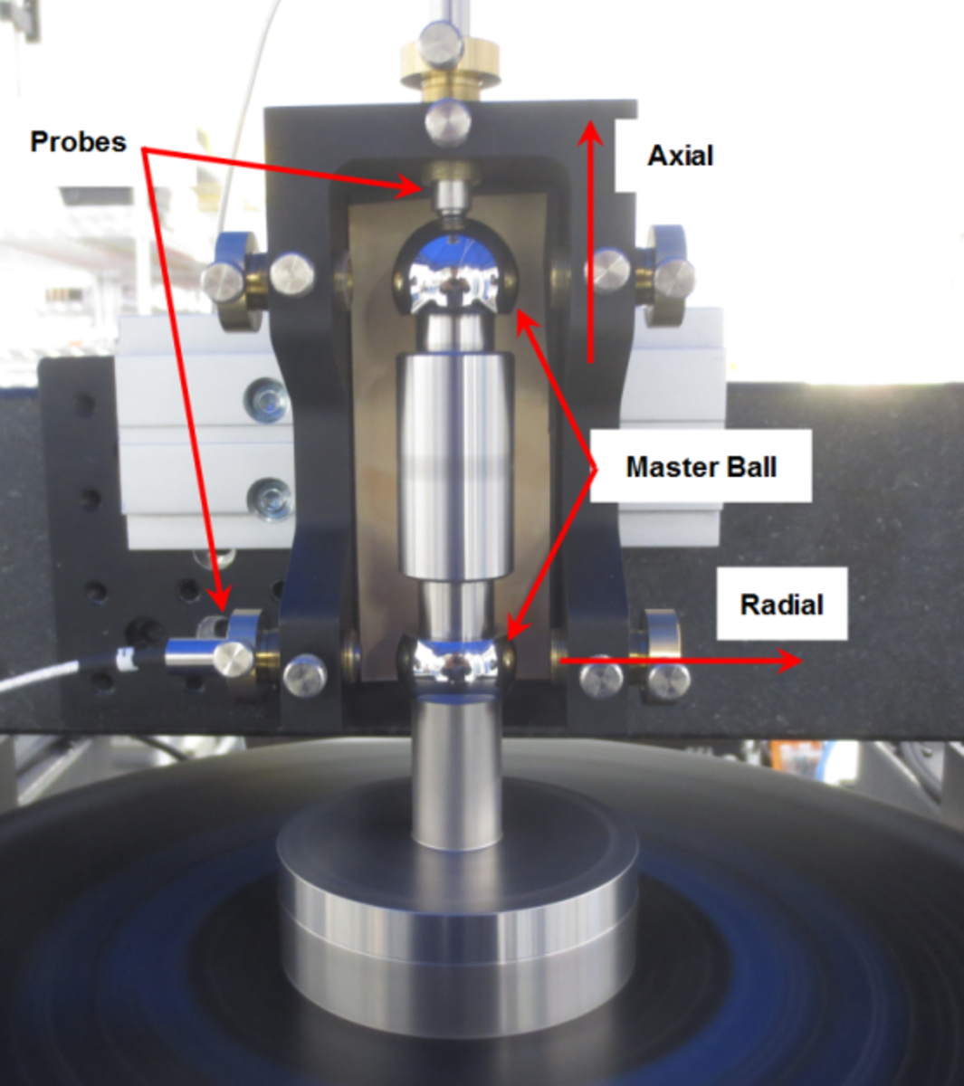
The tilt error motion setup is the same as the radial, except two balls and two probes measure radial error motion at the same time. Knowing the distance between the two probes, the angular error motion can be calculated.
Under closed loop servo control, the stage is rotated at a constant velocity while data is collected from the probes at a fixed rate (usually 100 Hz – 20 kHz). The stage is spun for several revolutions. The data that is collected is plotted and the overall error calculated. The results are reported in microns.
4. Limitations of Metrology
All of the tests described above can only measure one type of error motion at a time, one axis of motion at a time. Customers often ask us about “3D accuracy” or “overall precision.” Given the test methods we use, such specifications are difficult (if not impossible) to measure and therefore verify. We can make calculations to predict overall performance in average or worst-case scenarios, but we cannot verify those values with real work measurements.
Any metrology technique that can measure positioning errors in multiple degrees of freedom almost always depends on some sort of artifact, such a “golden wafer” or a “golden part.” Then a probe or a camera is used to measure the motion system’s ability to track or follow the master artifact. Such methods are comparative, depending on the known quality of the master artifact to verify overall performance. Since such artifacts are usually application specific, we don’t typically work with them at PI. Laser interferometer systems that measure multiple degrees of freedom at the same time do exist; however, these systems are usually used as control feedback system, not test metrology systems. And while they do measure multiple DOF at the same time, they are still only measuring individual errors, not true 2D or 3D spatial measurements.
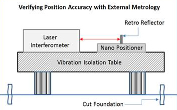
Precision metrology is incredibly sensitive to environmental conditions. The measurements we make at PI are under tightly controlled conditions. We isolate the system as much as possible from thermal variations, air currents, vibrations, audible noise, and electrical noise. Replicating the results in the field may be challenging.


Blog Categories
- Aero-Space
- Air Bearing Stages, Components, Systems
- Astronomy
- Automation, Nano-Automation
- Beamline Instrumentation
- Bio-Medical
- Hexapods
- Imaging & Microscopy
- Laser Machining, Processing
- Linear Actuators
- Linear Motor, Positioning System
- Metrology
- Microscopy
- Motorized Precision Positioners
- Multi-Axis Motion
- Nanopositioning
- Photonics
- Piezo Actuators, Motors
- Piezo Mechanics
- Piezo Transducers / Sensors
- Precision Machining
- Semicon
- Software Tools
- UHV Positioning Stage
- Voice Coil Linear Actuator
- X-Ray Spectroscopy